This page was generated from docs\source\gallery/Uflyand_Mindlin_matplotlib.ipynb.

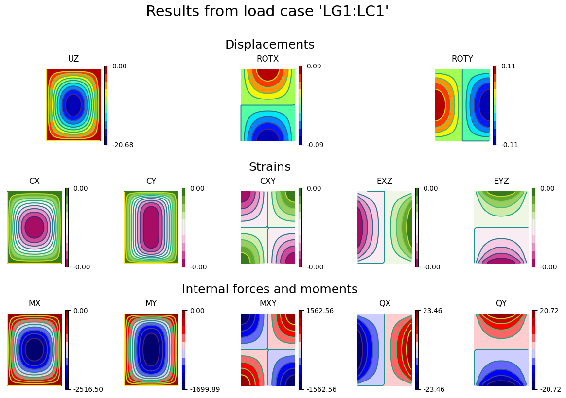
Contour plots of linear static analysis results for plates

Note

This example assumes that xarray, sigmaepsilon.solid.material and sigmaepsilon.mesh are installed.

import numpy as np
import matplotlib.pyplot as plt

from sigmaepsilon.math.linalg import ReferenceFrame
from sigmaepsilon.mesh.grid import grid
from sigmaepsilon.mesh import triangulate
from sigmaepsilon.mesh.utils.topology.tr import Q4_to_T3
from sigmaepsilon.mesh.plotting import triplot_mpl_data
from sigmaepsilon.solid.material import MindlinPlateSection as Section
from sigmaepsilon.solid.material import (
    ElasticityTensor,
    LinearElasticMaterial,
    HuberMisesHenckyFailureCriterion_SP,
)
from sigmaepsilon.solid.material.utils import elastic_stiffness_matrix

from sigmaepsilon.solid.fourier import (
    NavierPlate,
    LoadGroup,
    PointLoad,
    RectangleLoad,
)

# geometry
length_X, length_Y = (600.0, 800.0)
thickness = 25.0

# material properties
young_modulus = 2890.0
poisson_ratio = 0.2
yield_strength = 2.0

# solution parameters
number_of_modes_X = 20
number_of_modes_Y = 20

# setting up hooke's law
hooke = elastic_stiffness_matrix(E=young_modulus, NU=poisson_ratio)
frame = ReferenceFrame(dim=3)
stiffness = ElasticityTensor(hooke, frame=frame, tensorial=False)
failure_model = HuberMisesHenckyFailureCriterion_SP(yield_strength=yield_strength)
material = LinearElasticMaterial(stiffness=stiffness, failure_model=failure_model)
section = Section(
    layers=[
        Section.Layer(material=material, thickness=thickness),
    ]
)
ABDS_matrix = section.elastic_stiffness_matrix()
bending_stiffness, shear_stiffness = (
    np.ascontiguousarray(ABDS_matrix[:3, :3]),
    np.ascontiguousarray(ABDS_matrix[3:, 3:]),
)

# set up loads
loads = LoadGroup(
    LG1=LoadGroup(
        LC1=RectangleLoad([[0, 0], [length_X, length_Y]], [-0.1, 0, 0]),
        LC2=RectangleLoad(
            [[length_X / 3, length_Y / 2], [length_X / 2, 2 * length_Y / 3]],
            [-1, 0, 0],
        ),
    ),
    LG2=LoadGroup(
        LC3=PointLoad([length_X / 3, length_Y / 2], [-100.0, 0, 0]),
        LC4=PointLoad([2 * length_X / 3, length_Y / 2], [100.0, 0, 0]),
    ),
)
loads.lock()  # freezes the layout to protect agains typos

# set up plate
plate = NavierPlate(
    (length_X, length_Y),
    (number_of_modes_X, number_of_modes_Y),
    D=bending_stiffness,
    S=shear_stiffness,
)

# set up the grid for evaluation points and plotting
nx, ny = (30, 40)
evaluation_points, quads = grid(size=(length_X, length_Y), shape=(nx, ny), eshape="Q4")
evaluation_points, triangles = Q4_to_T3(evaluation_points, quads)
triobj = triangulate(points=evaluation_points[:, :2], triangles=triangles)[-1]

# calculate results
results = plate.linear_static_analysis(loads, evaluation_points)

# ------------------------------------------ plotting ------------------------------------------

plt.style.use("default")

fig = plt.figure(layout='constrained', figsize=(12, 8))
fig.suptitle("Results from load case 'LG1:LC1' \n", fontsize=22)
subfigs = fig.subfigures(3, 1, hspace=0.1)

# plotting the displacements
axs_top = subfigs[0].subplots(1, 3, sharey=True)
subfigs[0].set_facecolor("white")
subfigs[0].suptitle("Displacements", fontsize=18)
for i, key in enumerate(["UZ", "ROTX", "ROTY"]):
    triplot_mpl_data(
        triobj,
        ax=axs_top[i],
        fig=fig,
        title=key,
        data=results["LG1", "LC1"].to_xarray().loc[:, key].values,
        cmap="jet",
        axis="off",
        nlevels=10,
        lw=0
    )

# plotting strains
axs_middle = subfigs[1].subplots(1, 5, sharey=True)
subfigs[1].set_facecolor("white")
subfigs[1].suptitle("Strains", fontsize=18)
for i, key in enumerate(["CX", "CY", "CXY", "EXZ", "EYZ"]):
    triplot_mpl_data(
        triobj,
        ax=axs_middle[i],
        fig=fig,
        title=key,
        data=results["LG1", "LC1"].to_xarray().loc[:, key].values,
        cmap="PiYG",
        axis="off",
        nlevels=10,
        lw=0
    )

# plotting internal forces and moments
axs_bottom = subfigs[2].subplots(1, 5, sharey=True)
subfigs[2].set_facecolor("white")
subfigs[2].suptitle("Internal forces and moments", fontsize=18)
for i, key in enumerate(["MX", "MY", "MXY", "QX", "QY"]):
    triplot_mpl_data(
        triobj,
        ax=axs_bottom[i],
        fig=fig,
        title=key,
        data=results["LG1", "LC1"].to_xarray().loc[:, key].values,
        cmap="seismic",
        axis="off",
        nlevels=10,
        lw=0
    )

results["LG1", "LC1"].to_xarray().loc[:, "UZ"].values.shape

(1271,)